October 09, 2017
| · The third quarter GDP is likely to be distorted by the devastating impacts of Harvey and Irma, but the economic impacts from most natural disasters are temporary. With Federal aid, charitable donations and insurance payments, devastated areas will rebuild and grow again. From a fiscal spending standpoint, this is positive to the economy on the margin.
· Chair Yellen of the FOMC continues to hold the view that the current low inflation (however it is measured) is transitory and the FOMC is confident that it will rise to the 2% target level in the next year of two. Based on our analysis, survey-based inflation expectations (although lower than before) remain stable and the market-based measurements also suggest that the 2% target is within reach. Since consumer spending represents 70% of GDP, a lowering exchange rate will deliver supply-side inflation. More importantly is that we are all waiting for wages to grow at a faster pace (Phillips’ Curve discussion). This we believe is coming as unemployment continues to edge lower towards or pass NAIRU. These factors will likely contribute to reaching or passing the 2% target sooner – a positive for the economy on the margin. · President Trump’s crossing the political divide action to fund the government until December 15th and releasing the initial Hurricane assistance was a positive act (not considered so by the Republicans). This removed the Debt Ceiling debate (noise) from the 2018 budget/tax reform legislative agenda. Although it is not at all clear if President Trump’s proposed budget or the Big 6 negotiated tax reform will ever become law, there is an increasing sense of urgency to “do something” which could lead to compromise and constructive resolution in the months ahead. The market is again hopeful that something positive will pass for corporate America. On the margin, this is positive for the financial market. · The bias is for the FOMC to raise rates another 25bp in its December meeting. With the economy humming along, more new jobs being created, and the return of inflation, the FOMC is projecting three more hikes in 2018. Meanwhile, this month begins the balance sheet normalization process, albeit in tiny baby steps. In the near term, this should be well absorbed and understood by the market. Even with the ECB expected to pull back some of its bond buying, the world central bank balance sheets in the aggregate continue to grow. On the margin, this is positive/stable for the financial market. · What we worry about is the extended eerie calmness in the market. We hope that we are not simply under the “eye” of the storm while the devastating impact of a hurricane is around the bend. |
The U.S. Economy – Real GDP
The second quarter real GDP came in at 3% while the first quarter real GDP was revised up to 1.2%. The second estimate released at the end of August shows that consumer spending and capital expenditure by business were larger than previously estimated. However, these increases were partly offset by a larger decrease in state and local government spending. Our note, Behind the Headline – U.S. GDP 2nd Estimate[1], offers more details regarding the second estimate. For the first half of 2017, the real GDP is growing at a rate of 2.1%. To reach the higher watermark of 3%, the economy needs to grow at an average rate of 2.9% over the second half.
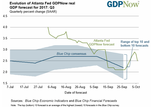
As of October 6th, the New York Fed’s Nowcasting projects the third quarter GDP to be at 1.53% while the Atlanta Fed’s GDPNow forecasts it to be at 2.5%.

Although the third quarter may have started well and continued the encouraging second quarter revised growth rate, the twin hurricanes of Harvey and Irma in late August and early September have, not only brought devastation and destruction to Texas and Florida, but created significant near term economic dislocation on these regions and affected the national GDP.
According to the FOMC September 20th Press Release: “Hurricanes Harvey, Irma, and Maria have devastated many communities, inflicting severe hardship. Storm-related disruptions and rebuilding will affect economic activity in the near term, but past experience suggests that the storms are unlikely to materially alter the course of the national economy over the medium term. Consequently, the Committee continues to expect that … economic activity will expand at a moderate pace”. The pre- and post-Harvey and Irma impacts are captured by First Data in its Economic Impact Analysis for Harvey[2] and separately for Irma[3]. The reports detail the consumer behavior in spending for building materials, gasoline, grocery, hotel, restaurant and travel before and after each hurricane. First Data’s press release, based on its data, affirms that “consumer spending in both impacted regions followed a similar trajectory. Spending increased the week before the hurricanes, with people stocking up on key items like gasoline and groceries, and dropped significantly during the storm. After the worst of the hurricanes, consumer spending rebounded as people began to rebuild.”[4] According to the Department of Commerce’s Bureau of Economic Analysis, as of 2016[5], the following is the current-dollar GDP by metropolitan area for the top 24 from the largest to the smallest.

| Total U.S. Metropolitan | $16,802,781 | 100% |
| Houston Metro Area | $478,618 | 2.85% |
| Miami Metro | $328,482 | 1.95% |
| Tampa Metro | $142,633 | 0.85% |
| Total | $949,733 | 5.65% |
According to this data, a portion of the 5.65% of the U.S. economy likely has been directly or indirectly affected because of the two hurricanes. This will materially impact the third and fourth quarter GDP. The question is the scope, scale and duration of this impact and the speed of access to money, cleanup, rebuilding and recovery. We expect these temporary factors will likely impact the GDP through the second quarter of 2018.
Many did not carry flood insurance, and the rebuilding will take time. Harvey damage is estimated at $150 billion or more. It temporarily shut down almost 25% of the oil and natural gas production and 10% of U.S. refining capacity. In the case of Irma, it wiped out much of the citrus groves’ production as Florida adds up its damages. Then, there is the latest Hurricane Maria devastating Puerto Rico.
We expect federal assistance of over $100 billion to be made available to all hard-hit areas. On the margin, this is an economic stimulus.
September is one of four times annually during which the FOMC publishes the Committee’s economic projections. The following graphs compare September and June FOMC Projection for the U.S. GDP going forward.


In its September release, the FOMC is projecting a medium GDP this year at 2.4% as compared to 2.2% in June. The projection for 2019 also moved higher to 2% from 1.9%.
It is often difficult to project GDP which is especially true when natural disasters are involved. We expect the 2017 real GDP to remain well within the 3% mark for which President Trump is hoping. We suspect the year will likely end in the 2.3% to 2.5% range which is right in line with the FOMC’s current projection. We are also in the camp that expects long-term GDP to remain below historical average due to low labor growth and productivity rates. Please refer to our commentary on this subject[6]. This does not mean there are no bouts of short term boosts to GDP due to fiscal stimulus and structural reforms. In fact, with the post hurricane fiscal injection, real GDP could be in the 3% or more annualized range for one or more quarters.
World Growth
There is no question that the world is growing at a faster pace than in 2016. The data provided by OECD for 2016 and 2017/2018 projections are summarized below:


These spider graphs easily show that there is increased economic growth in these countries from 2016 (blue) to 2017 (yellow) except for India. However, when comparing projected 2017 economic growth against 2018, the growth rate of change slows to negative.

Debt Ceiling and Tax Reform/Tax Cuts
There were two time-critical challenges facing the U.S. Congress as the summer vacation was coming to an end. The first was the issue of the debt ceiling, and the second was the 2018 budget. As always, Democrats and Republicans in today’s highly divided environment were expected to use these occasions to demonstrate their loyalty to their parties, make good on prior campaign promises, and put up a good fight for their ideology; all in the name of serving their constituent as they look nervously forward to the 2018 mid-term election. On September 6, President Trump took everyone by surprise and, to the chagrin of most Republicans, struck a deal with Democrats to increase the debt limit in order to finance the government until December 15 and to distribute $7.9 billion in emergency aid related to Harvey.
Currently, the government is operating under a temporary spending measure that runs out on December 8. And on October 5, the House of Representatives passed a 2018 budget resolution[7] via a 219-206 vote. All Democrats and 18 Republicans voted against it. The Senate Budget Committee[8] approved its alternative resolution on the same day. There are some major differences between the two versions, and the two chambers need to come to an agreement. Differences between the two budget resolutions must be negotiated, and the House and Senate need to agree to the same final bill. But this is really about tax reform. The budget is the prerequisite to using reconciliation for Republicans to push through a major tax bill. The fast-track procedure allows the Senate to pass a subsequent tax bill on a simple-majority vote rather than needing 60 votes. Although tax reform is not assured at all for 2017, the two chambers have taken the first step.

The market remains hopeful that some tax reform or tax cuts will happen this year and next year as a stimulus to the economy. The most likely or the least contested tax cut item is the tax holiday for corporations to repatriate their income to the U.S. at a one-time “discount” rate of 10%. This would generate much needed tax revenue and the repatriated capital would be positive for corporate America and the stock market.
Inflation: still missing the 2% target…for now
According to FOMC’s economic projections, the Committee continues to push its projection for the 2017 inflation rate while maintaining the 2% projection for 2019. The following graphs compare September and March meeting materials and summarize the FOMC’s projections for U.S. inflation (as measured by PCE) going forward. In the long-run, the Committee continues to project the 2% inflation target being met.


Over the 6-month period, the Committee lowered its median inflation projection by 0.3% from 1.9% to 1.6%. In fact, the 2018 medium projection has also moved down from 2% to 1.9%.
Inflation, or the lack thereof, continues to puzzle the FOMC. Quite frankly it is a conundrum. Although the observable factors contributing to low inflation are clear, it is not at all certain if the trend or the causation is transitory or if there has been a fundamental or systemic shift downward in inflation. After the economy and employment substantially recovered from the Great Recession, inflation remains elusive and somewhat surprising to the FOMC.
In Chair Yellen’s prepared remark after the September FOMC meeting, she said that “[f]or quite some time, inflation has been running below the Committee’s 2 percent longer-run objective. However, we believe this year’s shortfall in inflation primarily reflects developments that are largely unrelated to broader economic conditions. For example, one-off reductions earlier this year in certain categories of prices, such as wireless telephone services, are currently holding down inflation, but these effects should be transitory. Similarly, the recent, hurricane related increases in gasoline prices will likely boost inflation, but only temporarily… our understanding of the forces driving inflation is imperfect, and in light of the unexpected lower inflation readings this year, the Committee is monitoring inflation developments closely.” Subsequently in her response to question regarding inflation, she said: “I can’t say I can easily point to a sufficient set of factors that explain this year why inflation has been this low. I’ve mentioned a few idiosyncratic things, but frankly, the low inflation is more broad-based than just idiosyncratic things. The fact that inflation is unusually low this year does not mean that that’s going to continue. We’ve had several months of data that have meaningfully pulled that down, and what we need to do is figure out whether or not the factors that have lowered inflation are likely to prove persistent, or they’re likely to prove transitory, and that’s what we’re going to try to be determining on the basis of incoming data…”


Although the core CPI at 1.9% (monthly data of % change from one year ago, Seasonally Adjusted) is almost at the 2% Fed target, the Fed’s preferred gauge for inflation is the core Personal Consumption Expenditure (PCE) which is at 1.29%. (This is PCE minus food and energy.) It is clear that 2017 has been a falling inflation environment at a time of great consumer and business expectation and with an ever-shrinking unemployment rate. The expectation of more Americans back to work would naturally firm and ultimately drive up inflation. This would be what the Phillips Curve predicts, but inflation continues to trend down for now. Please refer to our recent commentary on this topic[9]. But the Phillips Curve relationship is not dead, it is simply delayed resulting from the ravages and policy/behavioral responses of the Great Recession and the Global Financial Crisis.
In her speech[10] at the National Association for Business Economics, on September 26th, Chair Yellen admitted that FOMC may have misjudged “the strength of the labor market, the degree to which longer run inflation expectations are consistent with our inflation objectives, or even fundamental forces driving inflation.” She considered the restraints imposed on inflation in recent years to be transitory factors including the movement in the relative prices of food, energy and imports as well as onetime events. These factors are expected to wane in the coming quarters. Even though inflation is still likely to stabilize at 2% over the next few years, the FOMC expects a high dispersion in its outcome. This uncertainty continues to be attributable to the price of oil, the exchange rate of the dollar and the idiosyncratic developments unrelated to the general economic conditions.

Although core PCI or core CPI remove the noisy or often volatile energy and food components of the underlying index, there are other refinements in looking at underlying indexes in an effort to be better informed about inflation. One way is to remove the volatile components (price changes) on both ends of the index to focus on those components that have moved the least during the measuring period. This is referred to as the trimmed mean PCE. The trimmed mean inflation rate is a proxy for true core PCE inflation rate. The resulting inflation measure has been shown to outperform the more conventional “excluding food and energy” measure as a gauge of core inflation.

The left graph compares the Trimmed Mean PCE inflation rate and the core inflation in the price index for PCE. The data series is calculated by the Dallas Fed, using data from BEA. Calculating the trimmed mean PCE inflation rate for a given month involves looking at the price changes for each of the individual components of PCE. The individual price changes are sorted in ascending order from “fell the most” to “rose the most,” and a certain fraction of the most extreme observations at both ends of the spectrum are thrown out or “trimmed”. The inflation rate is then calculated as a weighted average of the remaining components. In this case, as of the end of August, the Trimmed Mean PCE was at 1.38% as compared to the core PCE at 1.29%. Most of the time since 2000, the Trimmed Mean PCE is a bit higher than the Core PCE. Since the second quarter in 2016, the core PCE and the trimmed mean PCE have both trended downward to a cyclical low point.
Another way of dissecting the inflation data is to separate those CPI components with frequent price changes (Flexible CPI) from those components with slow price changes (Sticky CPI). According to Michael Bryan and Brent Meyer at the Federal Reserve Bank of Cleveland, their May 19, 2010, Economic Commentary article “Are Some Prices in the CPI More Forward Looking than Others? We Think So”[11] suggests that sticky prices appear to incorporate expectations about future inflation to a greater degree than prices that change on a frequent basis. Flexible prices, on the other hand, respond more powerfully to economic conditions— economic slack. Importantly, they found that sticky-price measure seems to contain a component of inflation expectations, and that component may be useful when trying to gauge where inflation is heading.
Sticky CPI represents those components of the CPI (approximately 70% of the CPI) with price change occurring less often, on average, than every 4.3 months. Flexible CPI (approximately 30% of the CPI) represents those components with a more frequent price change. The following are the sticky and flexible price components of the CPI used in the study:
| Flexible Price Components | Stick Price Components |
| Motor fuel | Infants’ and toddlers’ apparel |
| Car and truck rental | Household furnishings and operations |
| Fresh fruits and vegetables | Motor vehicle maintenance and repair |
| Fuel oil and other fuels | Motor vehicle insurance |
| Gas (piped) and electricity | Medical care commodities |
| Meats, poultry, fish, and eggs | Personal care products |
| Used cars and trucks | Alcoholic beverages |
| Leased cars and trucks | Recreation |
| New vehicles | Miscellaneous personal goods |
| Women’s and girls’ apparel | Communication |
| Dairy and related products | Public transportation |
| Nonalcoholic beverages, beverage materials | Tenants’ and household insurance |
| Lodging away from home | Food away from home |
| Processed fruits and vegetables | Rent of primary residence |
| Men’s and boys’ apparel | Education |
| Cereals and bakery products | Medical care services |
| Footwear | Water, sewer, trash collection services |
| Other food at home | Motor vehicle fees |
| Jewelry and watches | Personal care services |
| Motor vehicle parts and equipment | Miscellaneous personal services |
| Tobacco and smoking products |
The graph to the left plots the core CPI and Core PCE against the stick-price and flexible price components of the CPI since 2000. Currently, the Sticky CPI shows the highest annual change rate of 2.15% as compared to the core CPI at 1.7% and core PCE at 1.4%. Since December last year, there is a clear slide in inflation regardless of the measure. What is striking is the Flexible CPI where the latest annualized reading is at a negative 0.76%. The flexible price component of the CPI has been trending downward since February 2016. In fact, the Flexible CPI has been on a downward trajectory since the high (3.91%) reached in November 2011. It appears that what Chair Yellen refers to as “transitory factors” is likely referring to those impacting the flexible-price components of the CPI. However, the sticky-price components of the CPI appear to be fairly stable even though the prices have trended down since the beginning of this year. Many of the flexible-price components are made up of food and energy which are known to be volatile.

From a backward-looking standpoint, the Sticky or the Flex, the core, the headline, or the trimmed mean have all trended downwards in 2017. Chair Yellen has consistently attributed the recent drop in the inflation rate to transitory events (the Flex CPI components), but in reality, even the sticky components have trended lower. And the broad inflation indicator the FOMC focuses on is core PCE which is currently at 1.4% and far from the 2% target. From a forward-looking view, much of inflation is about expectation and examining consumer survey data, and professional market estimates could inform us about inflation sentiment.


The 5-year, 5-year Forward Inflation Expectation Rate measures the expected inflation rate (on average) over the five-year period that begins five years from today. The inflation expectation is now at 2.01% in Y2022. For a longer term look, we calculate the difference between the 10-year U.S. treasury Bond yield and the Treasury Inflation Protection Securities yield to see the “spread” which represents the inflation rate/compensation needed by the TIPS market. As of the end of September, this is at 1.8%.

The left graph illustrates the survey-based consumer inflation expectation. Based on the University of Michigan monthly surveys, the median expected price change for the next 12 months edged up in September to 2.7% from 2.6% in August. When looking at the combination of the market-based (professional) inflation expectation and the consumer-based survey results, it is clear that inflation expectation remains stable after drifting downwards in the recent past and the FOMC projections of core PCE reaching the 2% target in 2019 and beyond are in line with expectations.
In the very near term, inflation data will be noisy due to hurricane related spending and fiscal injections. However, in the intermediate term, there are increasing reasons to suggest that the 2% (maybe even higher) target will be reached.
Monetary Policy Normalization
In the September FOMC economic projections, the interest rate “dot plot” shows that, as 2017 is coming to an end, there is likely to be one more 25bp interest rate hike (from 8 in June to 11 members voting yes in September). The Committee is also looking to hike three more times next year as well (wide range) and bringing the Fed Fund rate to 2%.
| Midpoint of target range | 2017 | 2018 | 2019 | 2020 | Longer run |
| or target level (Percent) | |||||
| 1.000 | |||||
| 1.125 | 4(4) | 2(1) | 1(1) | 1 | |
| 1.250 | |||||
| 1.375 | 11(8) | ||||
| 1.500 | |||||
| 1.625 | 1(4) | 1 | 1(0) | ||
| 1.750 | |||||
| 1.875 | 2 | ||||
| 2.000 | |||||
| 2.125 | 6(5) | 1(0) | |||
| 2.250 | 1(0) | ||||
| 2.375 | 3(2) | 2(2) | 2 | ||
| 2.500 | 1(0) | 1(0) | 1 | 4(1) | |
| 2.625 | 1(3) | 2(3) | 2 | ||
| 2.750 | (1) | 1(0) | 1 | 4(5) | |
| 2.875 | 2(2) | 3 | |||
| 3.000 | (2) | 1 | 5(8) | ||
| 3.125 | (1) | 2(3) | 1 | ||
| 3.250 | 1(1) | ||||
| 3.375 | 2(1) | ||||
| 3.500 | 2 | 1(1) | |||
| 3.625 | 1 | ||||
| 3.750 | |||||
| 3.875 | 1 |

The above graph plots the FOMC Fed Fund rate projection against its core PCE projection over the next three years. For 2017, assuming inflation (core PCE) is at 1.5% and the rate by the end of this year is 1.4% (which is more likely to be 1.25%), we remain in a negative real rate environment. However, beginning in 2018 and going forward, the FOMC is projecting an increasing difference between the inflation rate and the Fed Fund rate. This suggests that the current FOMC members are looking to move back to a positive real rate environment beginning in 2019. If inflation exceeds the FOMC projections, the pace of raising rates may be even greater. The pace of normalization would likely speed up as well if the U.S. economy accelerates due to tax reform, tax cuts, fiscal spending, and stronger real wage growth. But for now, the probability of a 25bp rate increase in December this year, based on the CME Group Federal Funds Future contracts[12], is now at 98.5%; a virtual certainty.
The following graphs plots the 2-year treasury yield since 2000 and through the Global Financial Crisis. Since the first rate hike in December 2015 through the latest signalizing of a December 2017 rate hike, the 2-year yield has gone from 0.66% at the beginning of 2015 to 1.49% today. We think of the 2-year yield as the Risk Free Rate. During this period, the FOMC increased the Fed Fund rate from the 0.25% floor to 1.25% with the expectation of reaching 1.5% in December. The market is already priced in this final 2017 rate increase.

In the meantime, even as the 10-year treasury moved higher, the yield curve continues to flatten.

This month marks the much anticipated (since 2013 Bernanke Tapper Tantrum) balance sheet normalization. FOMC will commence balance sheet normalization using a cap system. The cap system limits the amount of principle reinvestment in treasury and agency securities over an 18-month period. According to the Fed’s published example under its Policy Normalization Q&A[13], the following two graphs illustrate the reduction or tapering process.


The upper left graph shows the monthly projected reinvestment in U.S. treasuries and the projected monthly “run-off” amount as scheduled. This does not include the reinvestment and run-off in mortgage based securities. This graph clearly shows that the balance sheet normalization is expected to be extremely gradual since there are still reinvestments from maturing securities above the caps.
Clearly, the Federal Reserve wants to carry out the normalization in an extremely gradual pace so that the well and transparent process of winding down the Large Scale Asset Purchase (“QE”) program is being carried out in the background systematically.
 In the foreseeable future, assuming all things equal, this pace and rate of normalization should have no discernable effect on the market. This is especially true when the ECB and the BOJ continue to expand their QE programs and the world would continue to be awash in central bank liquidity. In the next few quarters, the risk is likely to be on the upside for inflation, wage growth, and economic activities. With new FOMC members and the likelihood of a new Fed Chair, the certainty of the current normalization glidepath is called into question.
Are we too complacent under the “eye” of the storm?
After tropical storms Harvey, Irma, Jose, Maria, and now Nate, I can’t help but think if the financial markets are under the eye of a tropical storm. According to Wikipedia, the “eye” is a region of mostly calm weather at the center of strong tropical cyclones. The eye is surrounded by the eyewall, a ring of towering thunderstorms where the most severe weather and highest winds occur.
 First, the S&P500 has steadily risen (over 370%) since the low reach in March 2009 to the high in October 2017. At the same time, the Federal Reserve balance sheet has grown from less than $1 trillion to almost $4.5 trillion during the same period of time. This is not the only factor contributing to the market recovery since the Global Financial Crisis, but all the remaining observable factors are insufficient to explain the growth of the stock valuation.

 At the same time, the VIX is at historical lows. VIX is a measure of market expectation of near-term volatility conveyed by the S&P 500 option prices. The common explanation is the market is awash with (QE) liquidity and investors are pushed to take on risks in hopes of achieving expected returns. According to the CBOE, the average VIX value has been 18.73 since January 2, 2004, a 3,463-day period. In 2017, there were 26 days where VIX was below 10. This is almost half of the average or normal market volatility. It is interesting to note that, during the 2004 -2006 period, VIX was also below the historical average even though the FOMC had begun to raise interest rates. The projected three interest rate increases for 2018 (affecting short end of the yield curve) and the normalization of the Fed’s balance sheet (i.e. affecting the longer end of the yield curve) will continue to put upward pressure on interest rates. Initially, the market is expected to respond well to the broadcast rate increases, but as the chance of a policy error increases in anticipation or response to inflation or cyclical economic growth increases, this could quickly put pressure on risk assets as well as VIX.
The eerily low stock market volatility seems unsustainable. The graph[14] below shows that as of the end of Q3. There were only 8 days the S&P 500 Index had moved 1% or more in 2017. We have to go back to the mid 60’s to experience such a calm market…eye of the storm?

The St. Louis Fed Financial Stress Index[15] is at or near all-time lows as well.

The question is, with the gradual monetary policy normalization, at what point will volatility return?
Stable Disequilibrium Marches On
I have lost count of the number of times the Administration and the Republican-led Congress have failed to repeal and replace Obamacare. President Trump has again revived his efforts and is hoping for success. This is not simply about delivering on a campaign promise, it is about reclaiming $1 trillion in federal spending and repurposing it elsewhere. Since Trump’s win in November, the market has been hopeful for positive, pro-business changes. So far there have been no legislative wins but a lot of noise. The so call “Trump trade” waxed and waned aligning with the ever-changing efforts to “Make America Great Again.”
The executive branch has been successful in rolling back regulations where they can and continues to try to push for structural reforms. The latest is the Big 6 tax reform scheme. It is more a tax cut than reform and is another effort to rush through significant legislative changes in a compressed period of time. Ronald Reagan was the last President who successfully rewrote the tax code and implemented tax reform under two sets of legislations: the Economic Recovery Tax Act of 1981 and the Tax Reform Act of 1986. Regardless if we agree with the trickle down Reaganomics, it took President Reagan over 5-years of bi-partisan efforts to achieve tax reform. As such, whatever changes the current Administration can accomplish in 2017 would be small and are not likely to be tax reform and more likely a tax cut.
Regardless of intentions and politics, the current proposal is likely going to fail (or at the least be significantly modified) as well. But “hope springs eternal in the human breast,” the market remains hopeful that some tax relief will come to corporate America which would lead to a positive rippling effect in the economy. In the meantime, wages, productivity and GDP remain subpar. Although the central bank has taken credit through its unconventional monetary expansion policy for bringing America back to (almost) full employment, its other mandate of price stability remains shaky. With almost a decade of zero bound interest rates and quintupling its balance sheet, the biggest beneficiaries have been borrowers at the cost of savers and inflated financial assets. If we are in the eye of the storm where risks and tail events are unseen by us or market participants are not measuring the “right” factors, the tropical storm is likely all around us. We are nonetheless constructive about the U.S. and world economy. We know that the economic cycle (and the stock market) does not die of old age, but let’s hope that it is not done in by an aggressive or mis-stepping central bank.
Sincerely yours,
CHAO & COMPANY, LTD.
Philip Chao
Principal & CIO
This quarterly commentary represents the current views of Chao & Company, and they are subject to change. This Firm has no obligation or responsibility to update our views. The comments and views should not be deemed as Philip Chao, or any member of this Firm, offering personal or personalized investment advice. The quarterly commentary is informational only and is insufficient to be relied upon to make any financial or investment decisions or to make any changes to your financial condition.
[1] Behind the headline US GDP 2017 Q2 2nd Estimate/
[2] https://www.firstdata.com/newsroom/assets/Hurricane-Harvey-Economic-Impact-Analysis.pdf
[3] https://www.firstdata.com/newsroom/assets/Hurricane-Irma-Economic-Impact-Analysis.pdf
[4] https://www.firstdata.com/en_us/about-first-data/media/press-releases/09_22_17.html
[5] https://www.bea.gov/newsreleases/regional/gdp_metro/2017/pdf/gdp_metro0917.pdf
[6] Behind the Headline Is US GDP stuck in the low gear/
[7] https://budget.house.gov/budgets/fy18/
[8] https://www.budget.senate.gov/taxreform
[9] Behind the headline Phillips Curve/
[10] https://www.federalreserve.gov/newsevents/speech/yellen20170926a.htm
[11] https://www.clevelandfed.org/newsroom-and-events/publications/economic-commentary/economic-commentary-archives/2010-economic-commentaries/ec-201002-are-some-prices-in-the-cpi-more-forward-looking-than-others-we-think-so.aspx
[12] http://www.cmegroup.com/trading/interest-rates/countdown-to-fomc.html/
[13] https://www.federalreserve.gov/monetarypolicy/policy-normalization-qa.htm
[14] https://lplresearch.com/2017/10/02/where-did-all-the-big-moves-go/
[15] The STLFSI measures the degree of financial stress in the markets and is constructed from 18 weekly data series: seven interest rate series, six yield spreads and five other indicators. Each of these variables captures some aspect of financial stress. Accordingly, as the level of financial stress in the economy changes, the data series are likely to move together. The average value of the index, which begins in late 1993, is designed to be zero. Thus, zero is viewed as representing normal financial market conditions. Values below zero suggest below-average financial market stress, while values above zero suggest above-average financial market stress.